
How did the medium of the matrix come about?
Here are terms used, where are explained in Oscilllation of the matrix
It is arbitrarily assumed that we exist and that the universe has a
beginning. It is most likely not absolute. It is like the beginning of a day
based on the past day. After the birth of the universe, everything else is no
longer arbitrary but deterministic. In the beginning there will be a scenario
like the Big Bang of (more less than more) accepted theory. The unimaginable
forces, the extreme compression of space, immeasurable temperatures and a time
dilation into the infinite let expect that only configurations of a states of
highest harmony survived. In principle, the space itself found its most ideal
configuration, such as:
1.Tightest packing of space-structure
2. A cycle
of cascaded mini-cycles of time in (+) and (-) direction
3. The perfect
balance of compression / decompression momenta
In this way the universe could
present itself to the physicist as an empty space. No asymmetry of power, even
light was frozen in the perfect harmony of this configuration. After the universe
has start to expanded, the original configuration remained in the smallest cells,
then the gaps caused by the expansion were filled with new freedoms (according
to Feynman). These gaps became filled explosively with heat, light and motion.
The rest of the course is known to us. However, one event has not yet been
mentioned: the collapse of the rod resistances (the color distances) in the
order of M1; M2; M3 (metric of scales), which created the fermions as an
oscillation with vector to the 4th spatial dimension.
More info in matrix-4 scale 1
The Dynamic of the Matrix
The term MATRIX is a spatial network that consists of tetrahedral with
internal distances in the form of octahedral, is scalable, allows time to
act in two directions and has elasticity. Since it is assumed that
 physicists
also read with us, it should be noted that Euclidean space is generally used.
However, this is not isotropic and is used in the sense that in scale of
the particles with units of their rod lengths (color-distances), of the proton
(in the area of their collapse), in the area of fields with the
units of the metric (in the respective scale) and only in the area of EM-space
can be worked with quants in an Euclidean space. The spatial network of the
matrix is the basic structure in all areas, but its effects are becoming
less and less important with larger scales, its application ends with the
known analogue quantities, for which the relativistic space can be used as
required.
physicists
also read with us, it should be noted that Euclidean space is generally used.
However, this is not isotropic and is used in the sense that in scale of
the particles with units of their rod lengths (color-distances), of the proton
(in the area of their collapse), in the area of fields with the
units of the metric (in the respective scale) and only in the area of EM-space
can be worked with quants in an Euclidean space. The spatial network of the
matrix is the basic structure in all areas, but its effects are becoming
less and less important with larger scales, its application ends with the
known analogue quantities, for which the relativistic space can be used as
required.
Now some terms have already been used here, which are explained
in more detail in the Page MATRIX
The tetrahedron structure is explained in MATRIX Part 1. In the
sense of an equilibrium, only the tetrahedral are importand. The
octahedral are just gaps. In terms of the collapse of the rod lengths,
however, only the octahedral are considered, since it is their diagonals
that collapse. In physics they are called quarks.
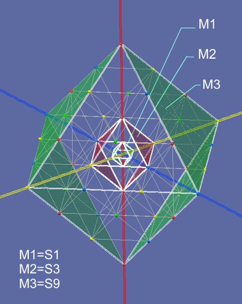
The size of space depends on the choice of its units. Apart from the
1 to1 representation of the rod lengths, the unit of which is the
diagonals of a S1-octahedron is shown as an proton. The field areas
around the proton are dependent on the scales M1; M2; M3 etc., which are
in a 3^x / 3^(x+1) relationship to each other and are based on the
structure of the superimposed octahedral; more in
Scales
The equilibrium in the tetrahedron area basically does not emit any
forces, the space is therefore called empty in the sense of normal
experiments. In this sense, space can also be viewed as isotropic. This
assumption provides correct results for the explanation of the charge
fields up to the material properties of matter.
The quantum structure remains in all size ranges. Basically, it shows effect in all scales, but is heavily overlaid by the analogues distribution effect in sense of 1/r^2. However, the scales can also take on any size up to astronomical ranges, making quantum effects theoretically possible in all ranges.
A quant is the momentum of h from pulses and length. Since the momentum h is invariable, the length is variable. This means that quantum quantities cannot be used as units of any order of magnitude. The quantities are related to each other in the ratio 3^x / 3^(x+1), ; M1; M2; M3; etc. are fixed sizes of space and apply to the subatomic range. This also automatically defines the pulse size of its metric.
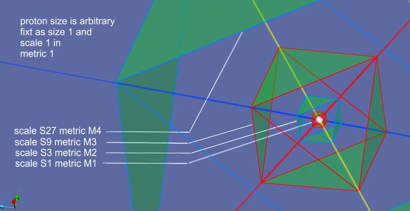
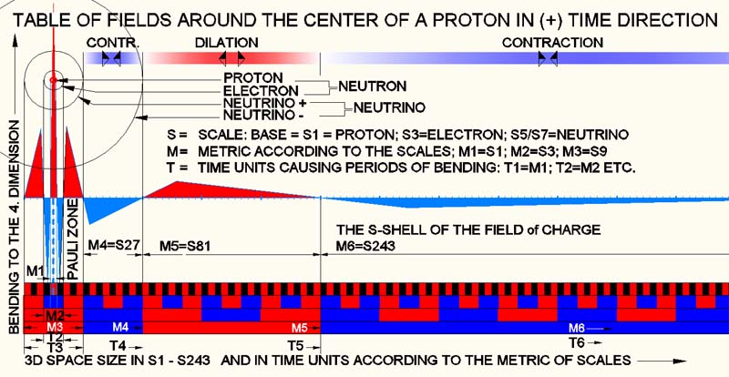
The picture above shows the different units of the different scales. The size of the pulse emitted by the oscillation of a proton in 3D space is fixed here as S1. S1 (λ) is therefore h/pulse. Pulse is not mc^2 here and should not be confused with the energies of this oscillation with vector in the 4th space dimension. It is only the side effect of this oscillation and only in 3D space of size M1. Since this can basically be aproached experimentally, a value should be found here. This is an invitation to physicists. Since S1 = M1 and the charge field of the S-shell is M6 = S243, a quant could be analyzed here and its length applied to the quantum S1. At the moment you can only think with relative values.
Do M1 cause a stack in lower sizes like M2 or M3
Here is an example: Given the frequency 10^10 for the oscillation of the proton, this creates a diffraction in 3D space, a quant with an associated frequency (S1=c/F) F=10^8. It will cause a stack of 10^10 - 10^8 = 10^2 quants. Here it is assumed that at the periphery of S1=M1=sphere=π•d^2=3 Quants of size S1 are emptied. From there the stack (100-3=97) will empty into M2=S3, where it will be emptied again at the periphery=sphere=π•d^2=27, if the quantum length is equal to (S1). Since in M2=S3 the length of the quantum is 3 times as long as Quant M1, the stack is only emptied by 27/3=9 quants. The time for the emptying is now seen 3 times longer, a compensation of this emptying in M1 is by 3•100=+300 quants, recovering the stack. With M3=S9 the emptying is π•9^2=254, the time belongs 9 times with a compensation in M1 of +900 quants. With M4 = S27 the emptying is π•27^2=2289, the compensation in M1 instead of 27•100=2700. It is stipulated that M5 and the emptying is greater than the compensation in M1
The example shows a major mistake in thinking, which is also based on one of the deepest secrets of QM (quantum mechanics). No energy flows from the oscillation of the proton. The interaction of the proton as an oscillation to the 4D space with the energies of the 3D space happened in principle much earlier, theoretically even when universe was born. It forms a fixed QM system, where the pulse sizes according to the metric they are in, having a fixed ratio, so that no energy is lost. An idealizing picture of “standing” waves can be imagined.
The hierarchy of fields
One can also speak of the hierarchy of standing waves.
First the term matrix in connection with field and wave.
The term matrix
consists of space-time and pulse, whereby pulse in its composite form also
means energy. In QT (quantum theory), the sizes or portions of space, time
and pulse are placed in a defined relationship. Each space no longer
consists of x, y, z, but rather of the units of space, a portion that is
also space and stands in certain harmonic relationships with the parent and
child space cells. This portion gets a reference value to the space of the
smallest field around the proton. E.g. the field with the metric M1 and the
size of scale S1. With the defined space portions, time and pulses are also
defined in accordance with the QT.
→ Time t = r/c where c = speed of
light and r = radius of the field size.
→ Pulse = h/r where h is the
Planck constant, r = radius of the field size.
Each space size therefore
has its own metric, time and pulse. The hierarchy of space sizes therefore
also results in a hierarchy of time and pulse sizes e.g. S9 = M3 corresponds
to its units time = T3 and pulse (M3).
The matrix is therefore not
just a spatial structure, but a harmonious interaktion of space, time and
pulse portions in the respective metric.
How to represent the geometry and metric of the matrix structure
I have to reminde that the matrix as a medium of the
univers and its fabrics consists of tetrahedral, which in their volume
filling result in a pattern of gaps with shapes of octahedral. This
results in an image that can be seen as a seamless space filling by
octahedral or by tetrahedral. The impact of the 4th spatial dimension force
us to see tetrahedral as carriers of spatial points of power, which as
equilibrium result in zero as a sum. The octahedral thus become the gaps in
space, which become a certain status value (++ + - - + -) in the collapse of
the structure. If the 3D space would be seen as a 2D surface, the collapsing
space into 4D space or into the n coordinate of the 4D space (x: y: z: n)
causes a bending in the 3D-surface.
Now we have to assigne the criteria time and
pulse or the momenta h to the structure. First, the 4 status values (++ +
- - + -) are assigned to the center points of space as 4 colors. The first
rules emerge:
• In sense of an equilibrium, no color can be the same
as its neighboring colors.
• In sine of spreading energy, each color
should be the same
The geometry of the matrix solve it like this:
If the space is filled with tetrahedral of side length S1 (arbitrary
assumption), then this length or rod length S1 results in a perfect
equilibrium. There, no color is the same as neighbour/colors.
If the side
length S2 is used in the same structure, the
same space status-color is always found for each space point. The space
becomes conductive for all disturbances caused by energy-differences. This
shows us what effect the distance between the points has. This is dealt in
detail in
Matrix Part 1
When explaining subatomic processes, the momentum h must now be introduced into the matrix structure as a universal constant. The players in this solution are the harmonic relationships of the individual frequencies. The term frequency was therefore already explained in the previous article and the link Oscillation . Each point in space or each color is an oscillation that is in a certain harmonic rhythm with neighboring colors. The frequency here is C-G-G´ or C-C´ in the sense of 12-tone music. This gives the aspect ratios of (-) to (+) e.g.
< < < 3^-4 ; 3^-3 ; 3^-2 ; 3^-1 ; 3^0 ; 3^1 ; 3^2 ; 3^3 ; 3^4 > > >
These distance ratios are subsequently referred to
as metrics. The reason for the introduction of the term metric is that for
the distances within the same metric there are the same conditions of the
rod lengths in such a way, that in every distance of the metric a status
change caused by V=c has the same effect as the original space cell.
E.g. red in distance x, the status will have changed to green, then all
neighboring colors will have also changed. It can thus be determined logically as
if there were simultaneities.
Each metric has a certain aspect ratio to
the neighboring metric in the direction of large and small. The lengths
correspond to ʎ = c/F, pulse = hc/ʎ and h = pulse ʎ/c.
On the thought way to explain particles and their cascaded fields in different metrics, a look at the geometry of matrix will be nessasary.
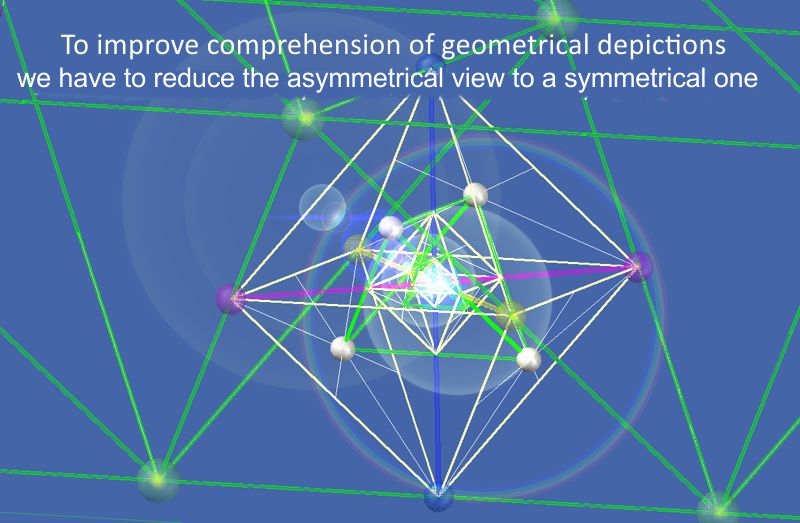
Here it becomes clear that an asymmetrical isometry images make it difficult to read the geometric laws. The display should show a symmetric isometry instead of an asymmetric one.
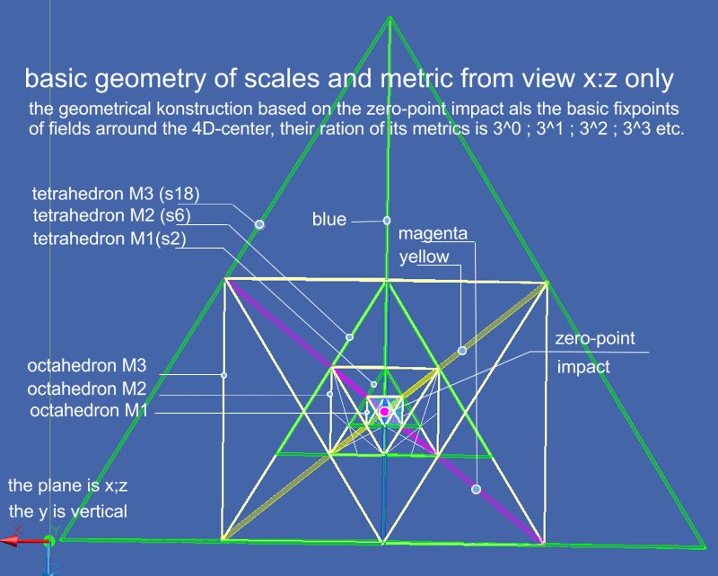
The second picture shows the octahedral in white, the tetrahedral in green from the coordinate position x; z and y as a perpendicular coordinate. The center in the geometric bodies is exactly at the same point in space. While the geometrically identical shapes are nested in each other, the octahedral of the same metric are touched by the tetrahedral of the smaller metric. The 3 diagonals of the octahedral are clearly visible with their 3 colors, here magenta-yellow-blue, which run unaltered and through each metric into the next higher one. It is recognized that all tetrahedral have the 4th color, here green. This only applies if the tetrahedral represent the maximum extent of a metric unit of an even space size like S2: S4: S6 etc. That is an important recognition: While the white octahedral represent a standing wave, the green tetrahedral are the pulse transmitting space.
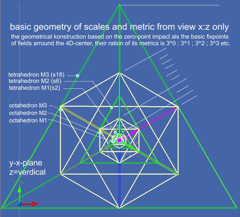
The third picture shows the spatial unit and its metric from y; x with z as the vertical coordinate. From this angle, the octahedral appear as hexagons and are nested symmetrically in each other.
How it comes to the picture of waves?
As described in the chapter Matrix / Oscillation, the 3D space can be
imagined as a surface with its vertical as a coordinate to the 4D space. At
the coordinates x; y; z, its z whould suppressed and replaced with "n" as a
vector for 4D space. Since 3D space is now a spatial structure, for
practical reasons the surface can be thought of as a thin fabric, the
network of which, like a knitted fabric with meshes of threads, can also be
partially imagined in the z direction (or here n). Each stitch is a
tetrahedron with 4 vertices (4 colors).
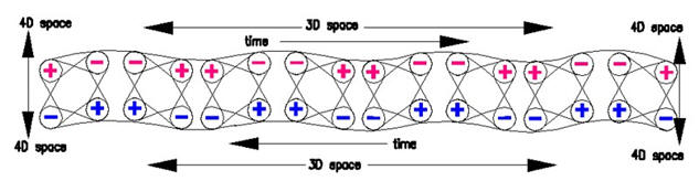
Thus the symbolic surface of the space becomes partially real. It gets a top and bottom. In our thought model, under certain circumstances, this surface can become bends in the form of waves. In this sense, the bends have an upper surface where the wave cress creates tensile stress and at the same time at lower surface, the bends generates compressive stress. That's exactly what happens in reality. The phenomena on the top generate the equivalent values on the bottom, a scenario of supersymmetry is shown here.
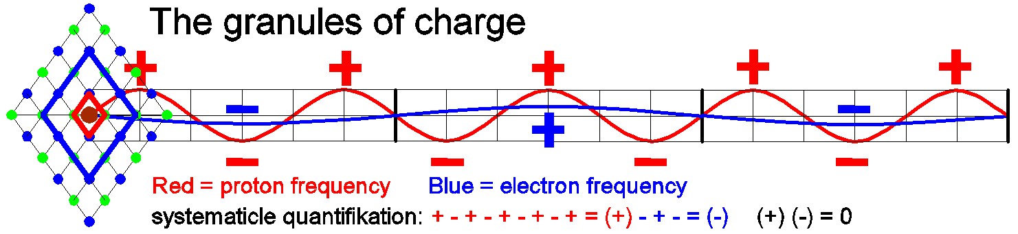
The picture shows on the left the space sizes M1 and M2 with the parities (+) and (-). In this example here is a proton inside a positron, i.e. represented a neutron. It symbolizes the ratio of the bends (waves): blue as M2 (S3) and red as M1 (S1) in a ratio of 3 to 1.
Space becomes properties and properties become space
With the assumption of a 4th spatial dimension, properties of 3D space can without it only be assigned to the particles and fields as arbitrary attributes. Here, with including the 4. dimension they can be explained. The 4th spatial dimension has a local impact on 3D space. Local (or standing) fields can be explained in this way, even if the medium of space would normally carry away any influence with V=c. The first field (M1) in 3D space is therefore the first secondary field and is generated by 3D space as its medium. The Planck constant in 4D space could be the same or different, it has no direct influence to 3D space. That means, a 4D-impact creates proper 3D-properties ruled by h.
Culmination (a wrong approach to Quantum Theory)
The first field M1 thus has its own time and frequency, which however, must
correspond to the frequency of the 4D pulse, even if the pulse does not
correspond to this frequency. In theory, an impact with a vector of 4D has
no direct influence, but its frequency does. A stacking of a quanta-effect,
however, would occur in the subsequent fields in a form similar to that
indicated in the chapter “The dynamics of the matrix”.
The fields around the 4D pulse in 3D space are therefore generated by two
causes.
1. From the QT dynamics, starting from the frequency of the
4D-impact.
2. From the stacking of the higher
frequency of the M1 in the following space-sizes.
Point 1 creates a field
hierarchy of harmonically graded amplitudes.
Point 2 creates a multiple
wave that pours from M1 to M2 to M3 etc. until there is entropy or equality
of space density with the surrounding fields. These two ways of generations
culminate and result in the hierarchy or constellation of fields arround a
particle. Despite point 2, the field relationships of the individual
particles can be compared without this stacking-effect, since this only influences
the amplitude of fields, but does not influence the
parities of these fields.
There is a big mistake hidden here !!!
There can´t be such culmination in QT of sub-particle size. Every change in frequency results in a spontaneous change in the field radius, which immediately compensates culminating of amplitudes. It is always a harmonic field hierarchy, ruled by h=pulse ▪ F/c. This special hierarchy of fields around particle corresponds to the geometrical constellation of the matrix as a local result of a zero-point impact from 4D-space. There a culmination of field-amplitudes causes spontaneous bending of hyperspace (4D). Any culmination is only possible by involving high energy in certain geometrical places. Even M1 field, caused by the 4D-Impact is fully ruled by h=pulse ▪ F/c.
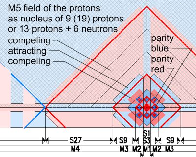
The picture shows the influence of the field parities of an atomic nucleus (atomic weight 19) and an electron on the S orbit or K shell. The expression "parity" is used here instead of "charge". That makes sense, since it is, as described in Matrix-charge, the bending of the 3D space what causes the attraction / repulsion effect. However, this bending is not static but oscillating. A smooth space cannot oscillate, but bending requires an oscillation.The oscillation, however, can have no charge. It is (+) and (-) . Since all spatial distances correlate harmoniously and have their own time and pulse with their own metrics, harmoniously staggered oscillations are possible. I.e. if two fields have the same parity (++) or (--), they repel each other, if they have a different parity (+ -) or (- +), they attract each other. With the hierarchy of space or field sizes and their own metric, the problem of V=c was also solved, since the hierarchies of the harmoniously nested space sizes have an interaction of the same or different parity and are therefore independent of time. This means that in large distances the large fields (M9; M10 etc.) are in effect and in small distances the small fields (M2; M3 etc.). Time only exists here for objects outside the oscillation and its metric.
What exactly does it mean?
All interactions happen as if they are simultaneous. Through the own metric
of space sizes M1; M2; M3; etc. there is no more time effect, only parities.
If e.g. a particle P1 (x1; y1; z1)
 interacts
with particle P2 (x2; y2; z2), P1 has the parity + and P2 has the parity -
then it doesn't matter where their fields are intersect. P1 can only
interact with the M3 of P2 with its own M3 field. The fields, regardless of
where, always interact with (+ -) or (- +) and are attracted in this case.
They change their values in pica seconds from (+ -) to (- +), their parity
always changes with the location, they are always attracted, regardless of
their oscillation status. Interacting always means a field overlay of the
same field size e.g. P1 by M4 and P2 by M4. Again in plain text: the
rhythm and oscillation of this kind of field (here the chargefield) is the
same in the whole universe. Although the
time delay by V=c is built in, it has no influence on the relation of the
status of field or their parities, since
particle oscillation does NOT
has a motion, but only propagates and is always an event of
the location. The connected properties such as charge are thus independent
of V=c and act as a permanent effect. That is the main reason, why to day's
physics think of charge as a permanent property.
interacts
with particle P2 (x2; y2; z2), P1 has the parity + and P2 has the parity -
then it doesn't matter where their fields are intersect. P1 can only
interact with the M3 of P2 with its own M3 field. The fields, regardless of
where, always interact with (+ -) or (- +) and are attracted in this case.
They change their values in pica seconds from (+ -) to (- +), their parity
always changes with the location, they are always attracted, regardless of
their oscillation status. Interacting always means a field overlay of the
same field size e.g. P1 by M4 and P2 by M4. Again in plain text: the
rhythm and oscillation of this kind of field (here the chargefield) is the
same in the whole universe. Although the
time delay by V=c is built in, it has no influence on the relation of the
status of field or their parities, since
particle oscillation does NOT
has a motion, but only propagates and is always an event of
the location. The connected properties such as charge are thus independent
of V=c and act as a permanent effect. That is the main reason, why to day's
physics think of charge as a permanent property.
Fields of protons
The bending of 3D-space effects first M1. M1 correlates with the
frequency corresponding to the 4D-impact (the 4D oscillation) (F = h/p), to
build up the metric. In short: a balance is formed already at
the birth of the universe (or when the proton is created). After that, no
energy flows. Any asymmetry would have dissolved already at the birth of the
universe. Only a perfect system whose values add up to zero would have
survived. In the case of a proton, this means (according to experiments) a
lifetime of 10^27 years, i.e. longer than the age of the universe it self
?!? The space sizes M1; M2: M3 etc. are basically empty quanta, which can be
filled "without penalty" without causing a flow of energies. The picture
above shows the cascades of the metric fields around a proton. These fields
are not only fields of activity in the 3D area, but also bends (as indicated
schematically with triangles) from the 4D-perspective. As described in
the link in matrix:
Oscillation.
They cause the bending (compression and decompression areas) in 3D-space. It
is the elasticity of the matrix as a medium that seeks balance in the
combinations of such (+) (-) areas, which causes the effect of
attraction or
repulsion instead of permanent given charge values (+) and (-). The (electrical) charge is
now explained as an parity, a quantum domain instead of being
arbitrarily determined for purely mathematical reasons.
Fields of electrons
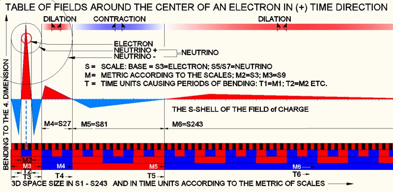 The
upper picture shows the schematic field representation of an electron. At
first glance, there is hardly any difference between the field division and
that of the proton. This is because the metrics of all fields are the same,
only the 4D-impact is different. The electron has its
momentum in M2 instead of M1 like the proton. Because M2 corresponds to the
time pulse T2, the
bending of the 3D-space at this point is opposite (contra-parity),
the momentum oscilates in opposite rhythm.
The
upper picture shows the schematic field representation of an electron. At
first glance, there is hardly any difference between the field division and
that of the proton. This is because the metrics of all fields are the same,
only the 4D-impact is different. The electron has its
momentum in M2 instead of M1 like the proton. Because M2 corresponds to the
time pulse T2, the
bending of the 3D-space at this point is opposite (contra-parity),
the momentum oscilates in opposite rhythm.
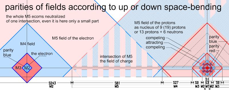
The Parity der Fields
Now a new scenario is looming: The fields (or more precisely: areas) which
are actually spherical around the 4D-impact (a point size), have parities in
form of certain frequencies correlating with the metric, since the 4D-impact
actually is an oscillation. Nevertheless, these frequencies can be
disregarded as they are compatible in themselves, i.e. a (+) field always
starts and ends with (+), even if the field is much larger. This effect was
marked with the lower bar black-
red
or blue-
red.
It should always be remembered that the matrix space consists of small
cycles of 4 colors as double oscillations,
which geometrically form the structure of the space as tetrahedral.
Therefore only certain constellation can apply, they all have to be done
according to the law of the MATRX, wich they exist from.
The above
pictures show areas of different parity of equal size. If you culminate
these areas eg. area of charge, then they result in zero, which in
reality means a smoothing of the 3-dimensional space. This smoothing of
space, on the other hand, relieves the tension of its elasticity
respectively relieves the tension in this area. This creates the effect of
attraction, which tends
to relieve space. The most important of these areas shown in the picture is
the area of charge. All attracting areas are separated from areas with
contra-parity, which in this case act as repulsions. These guarantee the
stability of such constellations. The area of charge is viewed in physics
as an EM space, because they are not yet ready to consider what happend in
these area is space and time,
They have the opinion, that an electron, a proton or other particl are
something separate from space. Here, however, all is only a state of the
matrix
respectively space-time-pulse.
Fields of the Neutron
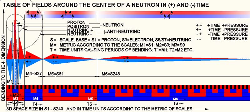 The
picture above shows the fields of a neutron. According to today's physics, a
neutron decays into a proton, a positron and an antineutrino during Beta-decay.
For this reason, I included a proton and an anti-electron (positron) in the
parity field table that we were able to see. I usually tried it with a
proton and an electron. But this would mean only a culmination of field
amplitudes. However, that wasn´t what I was looking for. The antielectron
culminated with M1 and M2 in bulk, that the compression part of the proton
in M1 was culminated with the M2 part of the antielectron, the part in M2
itself was equalized by the M2 part of the proton. Thus the culmination had
only a minimal effect instead. All other fields became equalized by the 3D-space
bending and didn't pass any values. The neutron was therefore minimally “heavier”,
but otherwise had no influence on local space warping (electrically neutral).
The
picture above shows the fields of a neutron. According to today's physics, a
neutron decays into a proton, a positron and an antineutrino during Beta-decay.
For this reason, I included a proton and an anti-electron (positron) in the
parity field table that we were able to see. I usually tried it with a
proton and an electron. But this would mean only a culmination of field
amplitudes. However, that wasn´t what I was looking for. The antielectron
culminated with M1 and M2 in bulk, that the compression part of the proton
in M1 was culminated with the M2 part of the antielectron, the part in M2
itself was equalized by the M2 part of the proton. Thus the culmination had
only a minimal effect instead. All other fields became equalized by the 3D-space
bending and didn't pass any values. The neutron was therefore minimally “heavier”,
but otherwise had no influence on local space warping (electrically neutral).
Here some thoughts about depiction
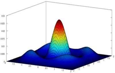 The
picture on the left shows space as x/y and the energy value as z. The colors
have no extra information, they only underline the z-values. With this
complex graphic very little can be represented . It could represent only
partial aspects of a particle, but not the anti-particle or its charge. No
relationships to quantum areas of the same size (metric) and no parities can
be shown. The theory remains an unrepresentable part. The upper
representation (table of fields) tries graphically to capture relationships
that were not previously made by the QM. The best representations in QM are
the Feynman graphs, which, however, only represent the theoretical results
in this way, but in reverse do not prove any such results.
The
picture on the left shows space as x/y and the energy value as z. The colors
have no extra information, they only underline the z-values. With this
complex graphic very little can be represented . It could represent only
partial aspects of a particle, but not the anti-particle or its charge. No
relationships to quantum areas of the same size (metric) and no parities can
be shown. The theory remains an unrepresentable part. The upper
representation (table of fields) tries graphically to capture relationships
that were not previously made by the QM. The best representations in QM are
the Feynman graphs, which, however, only represent the theoretical results
in this way, but in reverse do not prove any such results.
Paricle-physics as LHC result (Large Hadron Collider)
The discovery of electrons, protons, neutrons, neutrinos and their anti-parts had a long history. But recent discoveries of the debris in the rubble of cloud chambers in LHC have resulted in a rich yield of particles of all kinds. In the matrix theory, they are not directly detectable. Regardless of the expression particle - field - oscillation, it is clear that the above-mentioned particles are stable and have a lifespan of many years (proton = 10^27 years). However, their debris have a lifespan only of approx. 10^-20 (0.00000….) years and a trace of only few Ångström in the cloud chamber. The question now is whether these sparks can be called particles in the brutal high-energy experiments. It must be taken into account here, that the matrix structure in space-time-pulse as a geometric structure can also only produce debris with geometric quantum values. Chaotic and arbitrary values are not possible here. No wonder that the famous naming has resulted in a large number of (so called) particles. The theory presented here as Matrix resolves everything in parities, with attraction-repulsion being a parity of the diffraction of 3D space into hyperspace, the 4D-coordinate.
If you are interessted for a deeper insight to the Theory, read my papers for this subject.
Thr matrix of the medium of our world
The vibration of the world-medium
The geometry of the medium space
The universe
Friedmann-space and the space-matrix
The space-time continuum
The space- and time-illusion
Particle in the matrix structure
The Electron
Lützelflüh, the 20.12.2020 Switzerland